Interpreting Confusion Matrixes
Using standard metrics to interpret classification models in machine learning
Let’s say you’re running a classification experiment in machine learning and you have a trained model, but you want to understand how good that model actually is.
While there are a lot of different metrics and tools available to evaluate the performance of a classification experiment, the first one I always check is the confusion matrix.
Confusion matrixes give you an at-a-glance view of how a classification model tends to perform. It lets you quickly see where the model is strong and areas it might get things wrong a bit more than you’d like it to.
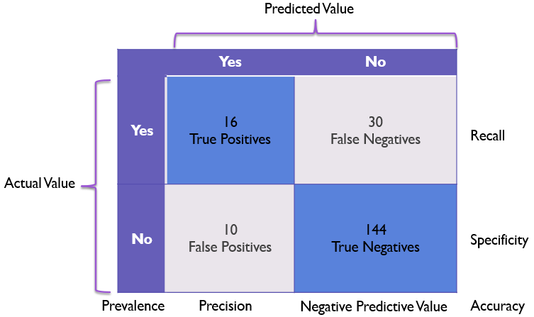
But confusion matrixes can be, well, confusing!
In this article we’ll explore confusion matrixes as well as related metrics in classification such as accuracy, precision, and recall. This article is an introductory one aimed specifically on binary classification, but I plan to follow up in the future with a more detailed article on multi-class classification.
This content is also available in video form on YouTube
Accuracy as a Simple Metric
Let’s say I’m performing a classification experiment to determine whether a painting was painted by Rembrandt or by someone else. I could train a classification model to evaluate information on the colors, brush strokes, age, and other factors to make a prediction as to whether a painting was likely to be a Rembrandt or was likely to be by any other artist. In this scenario, I’d be predicting a value of either 0 or 1. If the painting was likely to be a Rembrandt, the model should predict a 1. If it wasn’t the model should predict a 0.
I could evaluate the performance of this trained model with information on many paintings where I know definitively whether or not these paintings were by Rembrandt.
Let’s say I did this and gave the trained model 100 paintings of known origin to evaluate and it predicted correctly for 89 of them.
The simplest metric available to me is that this model is right 89% of the time or has an accuracy of 89% (sometimes written as 0.89 as a decimal percentage). This value can be calculated as follows:
accuracy = (true_positives + true_negatives) / num_observations
Here the term true positive refers to the number of times the model predicted a painting was a Rembrandt and it actually was and true negative refers to the number of times the model predicted a painting was not a Rembrandt when it wasn’t. In other words, we’re looking at the total number of correct categorizations divided by the total attempts.
Problems with Accuracy
However, accuracy can be misleading and can hide aspects of the full picture. For example, let’s say our sample data had only 11 Rembrandt paintings in it and all other paintings were by other artists. A simple model could predict that all paintings are not by Rembrandt and this model would still be right 89 times out of 100 (for every painting that is not by Rembrandt) and would appear to have an accuracy of 89%.
In this case our model is suffering from an alarmingly high number of false negatives where it states that a painting is not a Rembrandt where in reality it actually was.
Note: In statistics a false negative is sometimes referred to as a type 1 error or an alpha error
The inverse symptom would be a model with a high number of false positives where it predicted that every painting was a Rembrandt.
Note: In statistics a false positive is sometimes referred to as a type 2 error or a beta error
Clearly accuracy is not everything - particularly when you have imbalanced classes in your dataset where some classes occur less frequently than others.
Key Tip: Remembering the difference between true positives, false positives, true negatives, and false negatives can be difficult at first. An easy way to remember it is that the initial word of true or false refers to if our model made a correct or incorrect prediction whereas the last word of positive or negative refers to if the actual answer should have been yes or no
Confusion Matrixes to the Rescue
Confusion matrixes are a concise graphical way of displaying the true positives, true negatives, false positives, and false negatives in a model in a single table with actual values on the Y axis and predicted values on the X axis.
This would look something as follows:
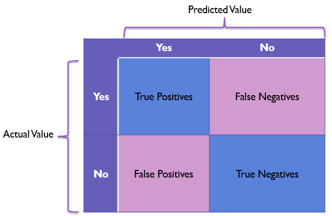
Note that the values on the diagonal from the top left to the bottom right are good predictions and the values on the diagonal from the top right to the bottom left are incorrect predictions.
Let’s get into a specific example with our Rembrandt painting scenario.
We’ll say we have a model that correctly identifies 16 Rembrandts (true positives) and 144 non-Rembrandts (true negatives), mistook 10 paintings as Rembrandts that were by other artists (false positives), and misidentified 30 Rembrandts as non-Rembrandts (false negatives).
The confusion matrix for this might look like the following:
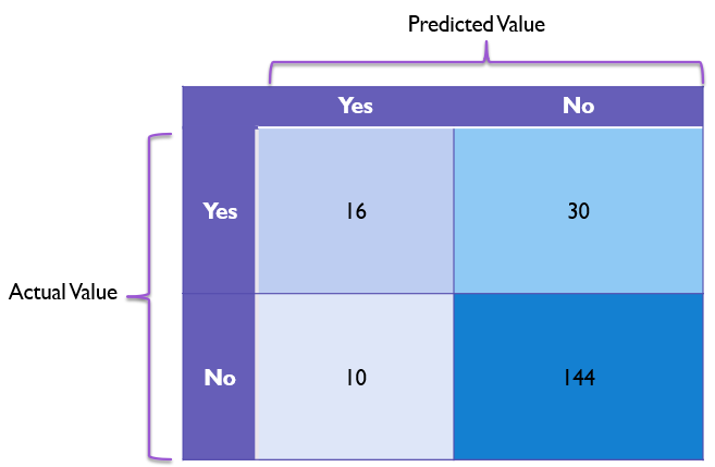
If we look at this confusion matrix, we can get a fairly good sense for where values tend to lay on this chart. This tells us at a moment’s glance that our model is good at identifying non-Rembrandts, but does have some notable problems recognizing Rembrandt paintings as actual Rembrandts.
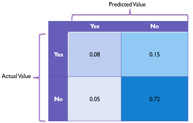
Sometimes it can be helpful to plot confusion matrixes as percentages of the whole in each box instead of the raw number of occurrences. An example of that with this data here would be as follows:
Revisiting Accuracy
In a confusion matrix, we can see the accuracy by looking at the values in the “correct” diagonal and dividing that total by the total number of observed values.
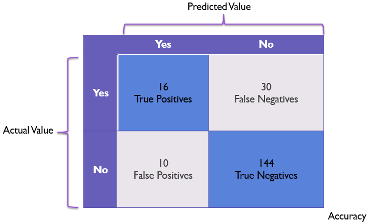
If all values are in the true positive or true negative boxes, our accuracy will be 100%.
Here we have 160 correct values (16 + 144) and a total of 200 values, giving us an accuracy of 160 / 200 or 80%. However, this accuracy rating doesn’t adequately convey the issues the model has with false negatives.
Recall
To address the issue of false negatives, we can turn to the metric of recall. Recall is the model’s ability to recognize positive values.
Note: Recall is sometimes also referred to as sensitivity
In our example recall means recognizing a Rembrandt painting as a Rembrandt, but in other examples it might mean flagging fraudulent transactions or correctly identifying cancerous moles as cancerous.
Recall can be calculated simply as follows:
recall = true_positives / (true_positives + false_negatives)
However, that can be hard to picture, so let’s look at this on our Confusion Matrix:
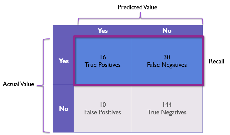
Here we focus on dividing the true positive cell divided by the count of the entire row where the actual value is positive.
In our example, this becomes 16 / 46 or 34.78%, which properly highlights the problems our model has at recognizing correct values.
However, recall is not inherently better than accuracy. For example, you could have a model that predicts that everything is positive. Such a model would have a recall of 100% and no false negatives whatsoever. To combat behavior like this, we rely on another metric: Precision.
Precision
While recall talks about our model’s ability to recognize positive values, precision is all about how reliable is a positive prediction from the model?
In other words, models with high precision are less likely to be wrong when they predict something as positive than models with low precision.
Precision is calculated as follows:
precision = true_positives / (true_positives + false_positives)
This can be visualized as the first column of the confusion matrix as follows:
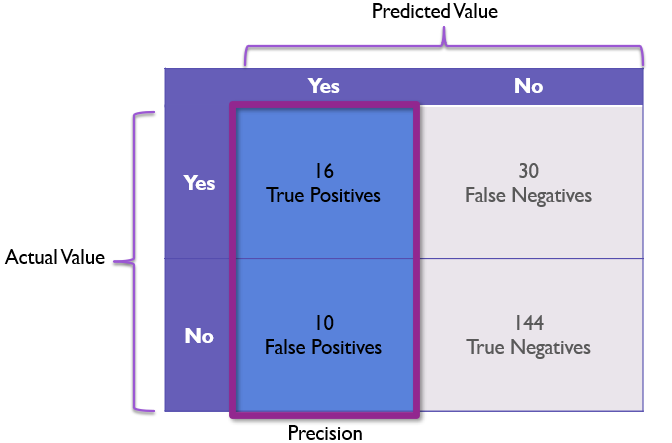
In our example, the precision would be 16/26 or 61.54%.
Specificity
Specificity is one I don’t see used as often, but it is almost the inverse of recall. While recall focuses on how reliable a yes prediction is, specificity focuses on how reliable a no prediction is.
Specificity is calculated as follows:
specificity = true_negative / (false_positive + true_negative)
This can be graphically represented on a confusion matrix as the bottom row:
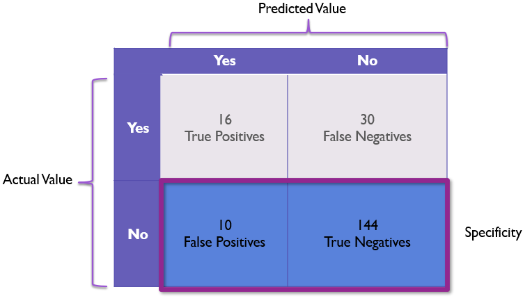
Here our specificity for the Rembrandt example would be 144 / 154 or a solid 93.51% giving us firm confidence in the model’s ability to identify non-Rembrandt paintings.
Negative Predictive Value (NPV)
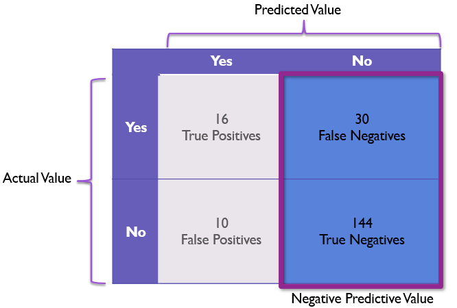
Negative Predictive Value or NPV is a term I don’t see frequently, but it is very similar to precision. While precision focuses on how much we can trust a positive prediction, NPV focuses on how reliable a negative prediction is.
We calculate NPV by dividing the correct negatives by the total negative predictions as follows:
npv = true_negative / (true_negative + false_negative)
In our example, this would be 144 / 174 or 82.75% meaning our negative values are mostly reliable, but our model still somewhat frequently rejects Rembrandt paintings as non-Rembrandt.
Prevalence
One final metric I want to point out is that of prevalence. Prevalence focuses on helping us identify class imbalances where one actual value is much more common than other values.
Prevalence is calculated as follows:
prevalence = (true_positives + false_negatives) / (false_positives + true_negatives)
In other words, in order to get prevalence of a given row we take the row and we divide it by the total items in the sample to get the prevalence of that type of item.
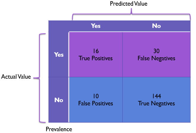
In binary classification (predicting only positive and negative values) models with prevalence values that are close to 50% are more evenly distributed and tend to have less issues than models with near 100% or near 0% prevalence values. For models with very low or very high prevalence values, precision and recall become more important to help balance against these class imbalances.
In our model we can calculate our prevalence as (16 + 30) / 200 or 46 / 200 which simplifies down to 23% for a somewhat imbalanced model with non-Rembrandts being more prevalent than Rembrandts.
Conclusion
Confusion matrixes are critical tools for analyzing the strengths and weaknesses of classification models.

At a simple level, confusion matrixes tell us how common different values are in our validation data, but as we’ve seen confusion matrixes also give us enough information to calculate accuracy, recall, precision, specificity, NPV, and prevalence for our model. All of this makes the confusion matrix the very first thing I look at when evaluating and communicating a classification model’s performance.
What constitutes a good model will be up to you and your team for the specific scenario that you are trying to solve.
For example, you will have to determine whether it is more important to have a high precision or a high recall (or if both are equally important). A cancer detection model might prioritize having a high recall so that cancer does not go undetected whereas a fraud detection model might prioritize precision to not penalize people flagged as false positives.
Ultimately, confusion matrixes give you a number of important metrics to solve classification problems - all wrapped up in a single diagram.


